Introduction

Il n’existe pas, à ma connaissance, de tutoriel complet sur TensorBoard, s’il y en a un il est bien caché et n’est sûrement pas en français.

Cet article a pour objectif de combler cette lacune.

magic commands : load_ext

L’appel de TensorBoard requiert l’utilisation de magic commands.

Pour rappel, concernant les magic commands :

Here we’ll begin discussing some of the enhancements that IPython adds on top of the normal Python syntax.

Here we’ll begin discussing some of the enhancements that IPython adds on top of the normal Python syntax.

These are known in IPython as magic commands, and are prefixed by the % character

These magic commands are designed to succinctly solve various common problems in standard data analysis. Magic commands come in two flavors: line magics, which are denoted by a single % prefix and operate on a single line of input, and cell magics, which are denoted by a double %% prefix and operate on multiple lines of input. 

Il faut tout d’abord « charger » TensorBoard

# Load the TensorBoard notebook extension
%load_ext tensorboard

Libération de l’espace de stockage

Les données enregistrées durant l’apprentissage (fit) sont stockées, enregistrées à l’endroit que vous spécifiez. Il est d’usage de commencer par supprimer toutes données antérieures.

Par exemple, en supposant que le dossier concerné est ./logs

# Clear any logs from previous runs
!rm -rf ./logs/ 

Exemple de modèle

Créons un modèle simple de classification MNIST

import tensorflow as tf
import datetime

mnist = tf.keras.datasets.mnist

(x_train, y_train),(x_test, y_test) = mnist.load_data()
x_train, x_test = x_train / 255.0, x_test / 255.0

def create_model():
  return tf.keras.models.Sequential([
    tf.keras.layers.Flatten(input_shape=(28, 28)),
    tf.keras.layers.Dense(512, activation='relu'),
    tf.keras.layers.Dropout(0.2),
    tf.keras.layers.Dense(10, activation='softmax')
  ])

model = create_model()
model.compile(optimizer='adam',
              loss='sparse_categorical_crossentropy',
              metrics=['accuracy'])

log_dir

Nous serons probablement amenés à exécuter plusieurs fois notre modèle. Raison pour laquelle, il faut un espace de stockage pour chaque run.

log_dir = "logs/fit/" + datetime.datetime.now().strftime("%Y%m%d-%H%M%S")
log_dir

Par exemple :

'logs/fit/20200917-104745'

callback

On définit ensuite un callback, une fonction qui sera appelée à chaque epoch (dans notre cas).

tensorboard_callback = tf.keras.callbacks.TensorBoard(log_dir=log_dir, histogram_freq=1)

fit

Lors du fit, on indique le callback (il peut y en avoir plusieurs)

model.fit(x=x_train, 
          y=y_train, 
          epochs=5, 
          validation_data=(x_test, y_test), 
          callbacks=[tensorboard_callback])

Visualisation

Des fichiers ont été créés durant le run d’apprentissage.

!ls -al $log_dir/train

total 72
drwxr-xr-x 3 root root  4096 Sep 17 11:59 .
drwxr-xr-x 4 root root  4096 Sep 17 12:00 ..
-rw-r--r-- 1 root root 54461 Sep 17 12:00 events.out.tfevents.1600343997.b0600510979a.102.162.v2
-rw-r--r-- 1 root root    40 Sep 17 11:59 events.out.tfevents.1600343999.b0600510979a.profile-empty
drwxr-xr-x 3 root root  4096 Sep 17 11:59 plugins

Ce sont ces fichiers que TensorBoard permet de visualiser.

Pour cela, utilisons la magic command %tensorboard en passant en paramètre le logdir :

%tensorboard --logdir logs/fit

Scalar

Par défaut, l’onglet visible dans le dashboard est scalar.

The Scalars dashboard shows how the loss and metrics change with every epoch. You can use it to also track training speed, learning rate, and other scalar values.

On peut ainsi consulter l’évolution de l’accuracy et de loss à chaque epoch.

Dans la colonne de gauche, il y a Smoothing défini de la façon suivante (raison pour laquelle il y a à chaque fois deux courbes lorsque smoothing est supérieur à 0)

It computes the exponential moving average over the list of data points. 

Si vous avez plusieurs run(s) vous pouvez préciser (à gauche) lesquels afficher.

Nous verrons plus loin comment ajouter d’autres données de type scalar à TensorBoard.

Graphs

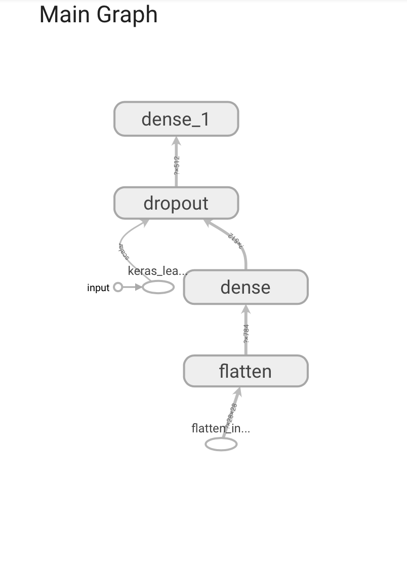
The Graphs dashboard helps you visualize your model. In this case, the Keras graph of layers is shown which can help you ensure it is built correctly.

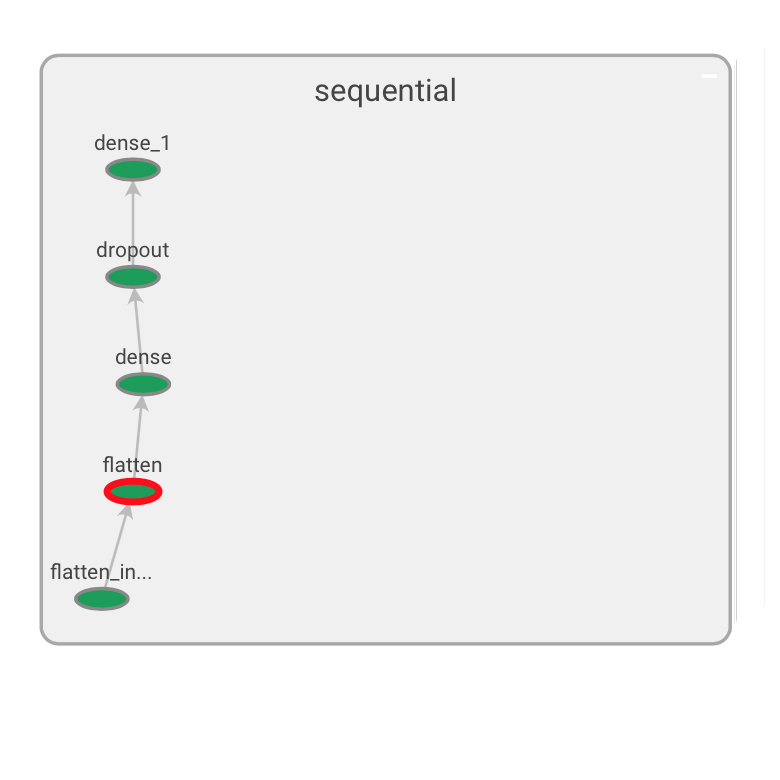
Par défaut, le graphe qui est présenté est op-level-graph (en comparaison avec le graphe conceptuel de type Keras).

Notez bien que les premières couches du réseau sont en bas (ce qui n’est pas intuitif !)

By default, TensorBoard displays the op-level graph. (On the left, you can see the “Default” tag selected.) Note that the graph is inverted; data flows from bottom to top, so it’s upside down compared to the code. However, you can see that the graph closely matches the Keras model definition, with extra edges to other computation nodes.

L’image est cliquable. Lorsqu’on positionne le curseur sur les éléments, un + s’affiche, ce qui permet de développer l’élément (la couche) étudié.

Par exemple, après avoir développé le flatten et le dense :

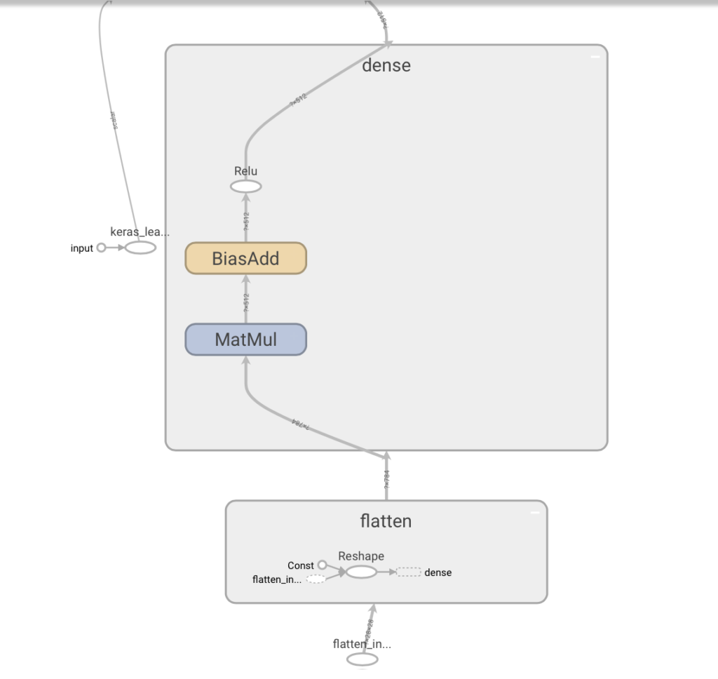
Les graphes peuvent aussi êtres présentés à la mode Keras (choisir cette option à gauche, tag = keras) et on peut même tester la compatibilité avec une exécution sur TPU.

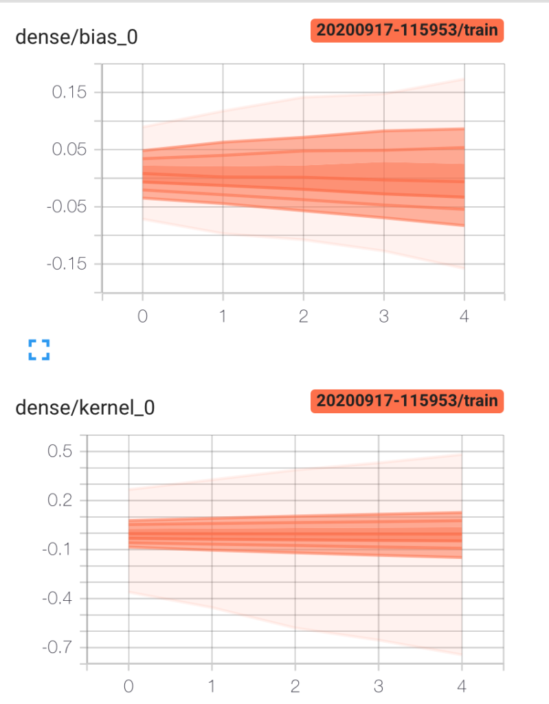
Distributions et Histogrammes

L’interprétation des histogrammes (qui ne sont pas des histogrammes) est difficile, c’est d’ailleurs aussi l’avis de l’équipe TensorBoard !

This histogram visualization is a bit weird, and cannot meaningfully represent multimodal distributions. We are currently working on a true-histogram replacement

https://github.com/tensorflow/tensorflow/blob/r0.9/tensorflow/tensorboard/README.md

The Distributions and Histograms dashboards show the distribution of a Tensor over time. This can be useful to visualize weights and biases and verify that they are changing in an expected way

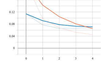
The Histogram Dashboard is for visualizing how the statistical distribution of a Tensor has varied over time. It visualizes data recorded via a tf.histogram_summary. Right now, its name is a bit of a misnomer, as it doesn’t show histograms; instead, it shows some high-level statistics on a distribution. Each line on the chart represents a percentile in the distribution over the data: for example, the bottom line shows how the minimum value has changed over time, and the line in the middle shows how the median has changed. Reading from top to bottom, the lines have the following meaning: [maximum, 93%, 84%, 69%, 50%, 31%, 16%, 7%, minimum]

https://github.com/tensorflow/tensorflow/blob/r0.9/tensorflow/tensorboard/README.md

Ce qu’il faut comprendre (à l’aide du schéma ci-dessous) :

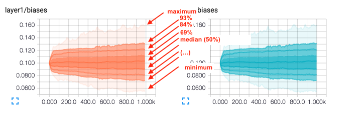
which means that the curve labeled 93% is the 93rd percentile, meaning that 93% of the observations were below the value ~0.130 at the time step 1.00k. So the graph gives 3 things of information, the percentage of observations bellow a certain value according to some think curve at every time step of the computation of the Neural network training (at least in this case its what the steps mean). This gives you a feel of the distribution of values of your network.

There are also the minimum and maximum values to get a sense of the range of values during training.

https://stats.stackexchange.com/questions/220491/how-does-one-interpret-histograms-given-by-tensorflow-in-tensorboard

Dans cet exemple, 93% des poids de la couche layer1, à l’epoch 1000, sont inférieurs à ~0.130.

Que fait-on de cette donnée ? donnée que l’on retrouve, différemment à l’onglet histograms. Ce n’est pas très clair !

Contrôle des enregistrements dans TensorBoard

La façon de procéder est différente. On contrôle la boucle avec tf.GradientTape() et les enregistrements avec tf.summary.

Dans cette version on choisit d’utiliser le Dataset.

import tensorflow as tf
import datetime
# Load the TensorBoard notebook extension
%load_ext tensorboard
# Clear any logs from previous runs
!rm -rf ./logs/ 

mnist = tf.keras.datasets.mnist

(x_train, y_train),(x_test, y_test) = mnist.load_data()
x_train, x_test = x_train / 255.0, x_test / 255.0

Les données numpy sont transformées en datasets.

train_dataset = tf.data.Dataset.from_tensor_slices((x_train, y_train))
test_dataset = tf.data.Dataset.from_tensor_slices((x_test, y_test))

train_dataset = train_dataset.shuffle(60000).batch(64)
test_dataset = test_dataset.batch(64)

Comme on contrôle la boucle d’apprentissage, on doit préciser les fonctions loss et les métriques.

loss_object = tf.keras.losses.SparseCategoricalCrossentropy()
optimizer = tf.keras.optimizers.Adam()

# Define our metrics
train_loss = tf.keras.metrics.Mean('train_loss', dtype=tf.float32)
train_accuracy = tf.keras.metrics.SparseCategoricalAccuracy('train_accuracy')
test_loss = tf.keras.metrics.Mean('test_loss', dtype=tf.float32)
test_accuracy = tf.keras.metrics.SparseCategoricalAccuracy('test_accuracy')

Fonctions training et test

tf.GradientTape() permet de créer un environnement dans lequel on trace les gradients.

On calcule la prédiction du modèle, on mesure la perte, puis on enregistre les gradients et enfin on les met à jour grâce à l’optimizer. Ensuite on calcule et enregistre les métriques.

La fonction de test est similaire sauf que bien sûr on ne calcule pas les gradients et a fortiori on ne les met pas à jour.

def train_step(model, optimizer, x_train, y_train):
  with tf.GradientTape() as tape:
    predictions = model(x_train, training=True)
    loss = loss_object(y_train, predictions)
  grads = tape.gradient(loss, model.trainable_variables)
  optimizer.apply_gradients(zip(grads, model.trainable_variables))

  train_loss(loss)
  train_accuracy(y_train, predictions)

def test_step(model, x_test, y_test):
  predictions = model(x_test)
  loss = loss_object(y_test, predictions)

  test_loss(loss)
  test_accuracy(y_test, predictions)

summary.writer

Le summary_writer nous permet d’écrire les données dans des fichiers compréhensibles par TensorBoard

current_time = datetime.datetime.now().strftime("%Y%m%d-%H%M%S")
train_log_dir = 'logs/gradient_tape/' + current_time + '/train'
test_log_dir = 'logs/gradient_tape/' + current_time + '/test'
train_summary_writer = tf.summary.create_file_writer(train_log_dir)
test_summary_writer = tf.summary.create_file_writer(test_log_dir)

Boucle

def create_model():
  return tf.keras.models.Sequential([
    tf.keras.layers.Flatten(input_shape=(28, 28)),
    tf.keras.layers.Dense(512, activation='relu'),
    tf.keras.layers.Dropout(0.2),
    tf.keras.layers.Dense(10, activation='softmax')
  ])

model = create_model() # reset our model

EPOCHS = 5

L’apprentissage consiste à itérer epochs fois, c’est à dire à parcourir l’ensemble des données epochs fois.

A chaque epoch, on effectue les calculs décrits plus haut et on enregistre les résultats. On le fait pour l’apprentissage et pour les données de test. On termine par un reset des métriques.

for epoch in range(EPOCHS):
  for (x_train, y_train) in train_dataset:
    train_step(model, optimizer, x_train, y_train)
  with train_summary_writer.as_default():
    tf.summary.scalar('loss', train_loss.result(), step=epoch)
    tf.summary.scalar('accuracy', train_accuracy.result(), step=epoch)

  for (x_test, y_test) in test_dataset:
    test_step(model, x_test, y_test)
  with test_summary_writer.as_default():
    tf.summary.scalar('loss', test_loss.result(), step=epoch)
    tf.summary.scalar('accuracy', test_accuracy.result(), step=epoch)
  
  template = 'Epoch {}, Loss: {}, Accuracy: {}, Test Loss: {}, Test Accuracy: {}'
  print (template.format(epoch+1,
                         train_loss.result(), 
                         train_accuracy.result()*100,
                         test_loss.result(), 
                         test_accuracy.result()*100))

  # Reset metrics every epoch
  train_loss.reset_states()
  test_loss.reset_states()
  train_accuracy.reset_states()
  test_accuracy.reset_states()

On peut ensuite afficher les données avec TensorBoard

%tensorboard --logdir logs/gradient_tape

Enregistrement de scalaires définis par soi-même

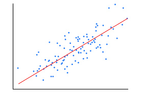
Prenons l’exemple d’une régression linéaire.

# Load the TensorBoard notebook extension.
%load_ext tensorboard

from datetime import datetime
import tensorflow as tf
from tensorflow import keras

import numpy as np

print("TensorFlow version: ", tf.__version__)

La création des données est la suivante :

import matplotlib.pyplot as plt
data_size = 1000
# 80% of the data is for training.
train_pct = 0.8
train_size = int(data_size * train_pct)
# Create some input data between -1 and 1 and randomize it.
x = np.linspace(-1, 1, data_size)
np.random.shuffle(x)
# Generate the output data.
# y = 0.5x + 2 + noise
y = 0.5 * x + 2 + np.random.normal(0, 0.05, (data_size, ))
# Split into test and train pairs.
x_train, y_train = x[:train_size], y[:train_size]
x_test, y_test = x[train_size:], y[train_size:]
# Clear any logs from previous runs
!rm -rf ./logs/ 

On utilise  tf.summary  qui permet d’enregistrer les données résumées.

logdir = "logs/scalars/" + datetime.now().strftime("%Y%m%d-%H%M%S")
file_writer = tf.summary.create_file_writer(logdir + "/metrics")
file_writer.set_as_default()

La fonction de calcul du learning rate :

def lr_schedule(epoch):
  """
  Returns a custom learning rate that decreases as epochs progress.
  """
  learning_rate = 0.2
  if epoch > 10:
    learning_rate = 0.02
  if epoch > 20:
    learning_rate = 0.01
  if epoch > 50:
    learning_rate = 0.005

  tf.summary.scalar('learning rate', data=learning_rate, step=epoch)
  return learning_rate

lr_callback = keras.callbacks.LearningRateScheduler(lr_schedule)
tensorboard_callback = keras.callbacks.TensorBoard(log_dir=logdir)

On a 2 callback, le 1er pour le calcul du learning rate, le second pour l’enregistrement des données pour TensorBoard

model = keras.models.Sequential([
    keras.layers.Dense(16, input_dim=1),
    keras.layers.Dense(1),
])

model.compile(
    loss='mse', # keras.losses.mean_squared_error
    optimizer=keras.optimizers.SGD(),

training_history = model.fit(
    x_train, # input
    y_train, # output
    batch_size=train_size,
    verbose=0, # Suppress chatty output; use Tensorboard instead
    epochs=100,
    validation_data=(x_test, y_test),
    callbacks=[tensorboard_callback, lr_callback],
)

%tensorboard --logdir logs/scalars

Dans l’onglet scalars, s’affiche les données

Réglage des hyperparamètres

Les nouvelles versions de TensorBoard permettent désormais de faciliter le tuning des hyperparamètres.

On fait le test sur fashion MNIST

# Load the TensorBoard notebook extension
%load_ext tensorboard
# Clear any logs from previous runs
!rm -rf ./logs/ 

On importe hparams.

import tensorflow as tf
from tensorboard.plugins.hparams import api as hp

fashion_mnist = tf.keras.datasets.fashion_mnist

(x_train, y_train),(x_test, y_test) = fashion_mnist.load_data()
x_train, x_test = x_train / 255.0, x_test / 255.0

On choisit nos hyperparamètres, on précise le nom et l’étendue des valeurs

HP_NUM_UNITS = hp.HParam('num_units', hp.Discrete([16, 32]))
HP_DROPOUT = hp.HParam('dropout', hp.RealInterval(0.1, 0.2))
HP_OPTIMIZER = hp.HParam('optimizer', hp.Discrete(['adam', 'sgd']))

METRIC_ACCURACY = 'accuracy'

On crée un filewriter qui mémorisera les paramètres en cours d’exécution.

with tf.summary.create_file_writer('logs/hparam_tuning').as_default():
  hp.hparams_config(
    hparams=[HP_NUM_UNITS, HP_DROPOUT, HP_OPTIMIZER],
    metrics=[hp.Metric(METRIC_ACCURACY, display_name='Accuracy')],
  )

Le modèle est classique. A la différence des autres, il est paramètré.

Partout ou il y a des paramètres à tester, on utilise hparams. C’est la seule différence.

def train_test_model(hparams):
  model = tf.keras.models.Sequential([
    tf.keras.layers.Flatten(),
    tf.keras.layers.Dense(hparams[HP_NUM_UNITS], activation=tf.nn.relu),
    tf.keras.layers.Dropout(hparams[HP_DROPOUT]),
    tf.keras.layers.Dense(10, activation=tf.nn.softmax),
  ])
  model.compile(
      optimizer=hparams[HP_OPTIMIZER],
      loss='sparse_categorical_crossentropy',
      metrics=['accuracy'],
  )

  model.fit(x_train, y_train, epochs=1) # Run with 1 epoch to speed things up for demo purposes
  _, accuracy = model.evaluate(x_test, y_test)
  return accuracy

Puisqu’on veut enregistre les données dans TensorBoard, on doit se servir du file_writer.

def run(run_dir, hparams):
  with tf.summary.create_file_writer(run_dir).as_default():
    hp.hparams(hparams)  # record the values used in this trial
    accuracy = train_test_model(hparams)
    tf.summary.scalar(METRIC_ACCURACY, accuracy, step=1)

L’exécution peut se coder de la façon suivante :

session_num = 0

for num_units in HP_NUM_UNITS.domain.values:
  for dropout_rate in (HP_DROPOUT.domain.min_value, HP_DROPOUT.domain.max_value):
    for optimizer in HP_OPTIMIZER.domain.values:
      hparams = {
          HP_NUM_UNITS: num_units,
          HP_DROPOUT: dropout_rate,
          HP_OPTIMIZER: optimizer,
      }
      run_name = "run-%d" % session_num
      print('--- Starting trial: %s' % run_name)
      print({h.name: hparams[h] for h in hparams})
      run('logs/hparam_tuning/' + run_name, hparams)
      session_num += 1

Puis :

%tensorboard --logdir logs/hparam_tuning

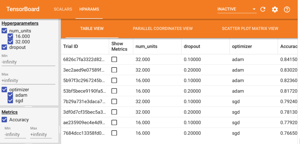
Le meilleur résultat est avec 32 units, dropout=0,1 et optimizer=adam.